Integration Rejection: Choosing an Algorithm and Reading the Rejection Map

When you integrate multiple frames, “rejection” is the process of automatically discarding the outliers that shouldn’t be there — satellite trails, cosmic-ray white spots, leftover hot pixels, the bloated halos around overly bright stars, and so on. Choosing the right rejection algorithm and knowing how to read the maps it produces is the key to a clean integration. This article lays out the logic behind choosing a rejection algorithm, plus exactly how to read those two rejection maps that so often get ignored.

The Family of Rejection Algorithms

PixInsight offers several rejection algorithms during integration. The official documentation lists which algorithm suits which scenario, and it’s well worth a read (note that this document was published a while ago and doesn’t cover the GESD algorithm that was added later).

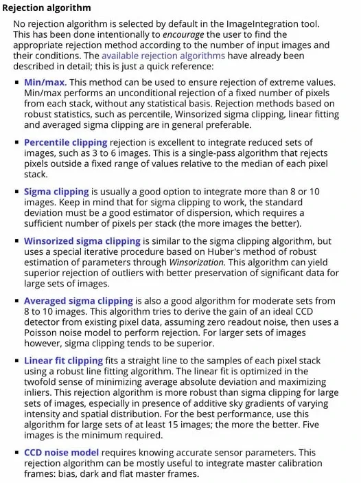
The rejection algorithms listed in the PixInsight Image Integration documentation

They fall roughly into two categories:

The Sigma family: outlier rejection based on standard deviation — for example Sigma Clipping, the improved Winsorized Sigma Clipping, and Percentile Clipping. Their underlying principles and mathematics belong to the same system.
GESD Test: based on Grubbs’s test, its theory and mathematics are completely different from the sigma-based methods. It’s a relatively recent addition.

GESD vs Sigma: Who Wins With Few Frames?

I’ve actually run the comparison. One time I took a dataset of only 12 frames and ran GESD Test, Winsorized Sigma Clipping, and traditional Sigma Clipping side by side.

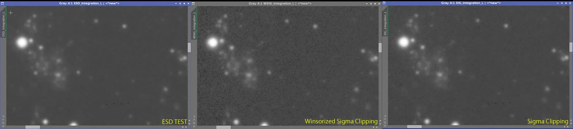
Comparison of GESD, Winsorized Sigma, and Sigma Clipping (12-frame dataset)

Twelve frames actually doesn’t meet the recommended frame count for GESD or Winsorized Sigma, yet in this particular set GESD Test gave the best result. But one caveat to add as a footnote: if you’re dealing with color data and too few frames, Winsorized Sigma or Sigma is still the better choice. So there’s no algorithm that’s “always best” — it depends on the data.

GESD Against Faint Satellite Trails

GESD has another practical advantage. Back when I integrated with the sigma family, I often ran into faint satellite trails that just wouldn’t reject — even with 17 frames, part of the trail would still remain after integration, and this kind of faint trail isn’t suited to manual selective rejection (painting it black).

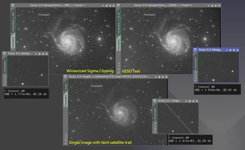
Successful rejection of a faint satellite trail after adjusting GESD parameters and growing the trail

Switching to GESD Test, and appropriately adjusting the parameters and growing (dilating) the faint satellite trail, I successfully rejected an extremely faint trail; and generally speaking, GESD’s signal-to-noise ratio is higher than traditional Sigma Clipping or Winsorized Sigma Clipping. (That said, in most cases you won’t hit this un-rejectable problem with the sigma family — this is a fairly extreme edge case.)

A Special Weapon: Range Clipping

Besides statistical outlier rejection, there’s another “brute-force” but handy tool — Range Clipping.

Using Low Range clipping to forcibly remove black spots caused by poor dark calibration

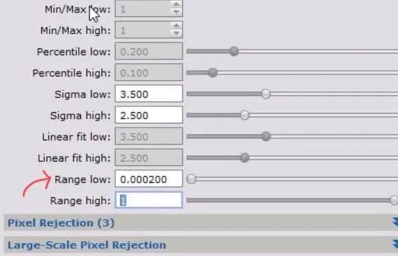
If you have frames with poor dark calibration that show lots of black spots (say, present in 10 frames, absent in 5), the regular rejection algorithms struggle to remove these black spots by picking outliers. In that case you can use Range Low Clipping during integration to forcibly remove every black spot below a certain threshold. It’s a direct tool aimed at a specific defect, complementary to statistical rejection.

The effect of Low Range clipping removing the black spots

Reading the Rejection Map

When you integrate with ImageIntegration or WBPP, besides the finished image you also get two rejection maps: one for the high-brightness direction (rejection high) and one for the low-brightness direction (rejection low). Most people simply ignore these two — which really wastes some very useful diagnostic information.

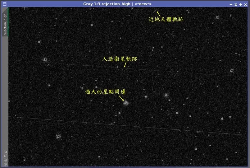
Satellite trails, bloated star halos, and near-Earth object trails appearing in the rejection high map

Usually there’s not much to see in rejection low; the interesting one is rejection high: this is where all the interference you’d rather “not appear in the finished image” shows up — satellite trails, the halos of overly bright or bloated stars, near-Earth object trails, plus hot pixels and cosmic-ray white spots (I usually clean hot pixels out with Cosmetic Correction before integration, so there aren’t many here).

The most practical way to read this map is: if a pixel you wanted rejected shows up in rejection high, it means it was successfully removed; if it doesn’t show up here yet remains in the integrated result (for example a leftover satellite trail), it means your rejection parameters aren’t strong enough, or you should switch algorithms.

A Few Common “Should I Drop This Frame?” Questions

Once you understand the principles above, a lot of the things beginners agonize over have clear answers.

A frame with bloated stars — should I drop it from integration? Unless it’s out of focus, I usually let it participate in the integration.

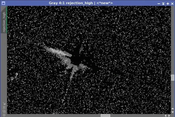
Illustration of bloated / overly bright star halos and satellite trails being rejected in rejection high

Inspect the rejection high map and you’ll see that the oversized or overly bright parts of those stars have already been removed by rejection and didn’t take part in the integration math; satellite trails and cosmic-ray white blobs likewise land in rejection high. Just let the software handle this kind of work.

A bright satellite trail cuts right across the target — should I manually delete that frame? The answer is again no.

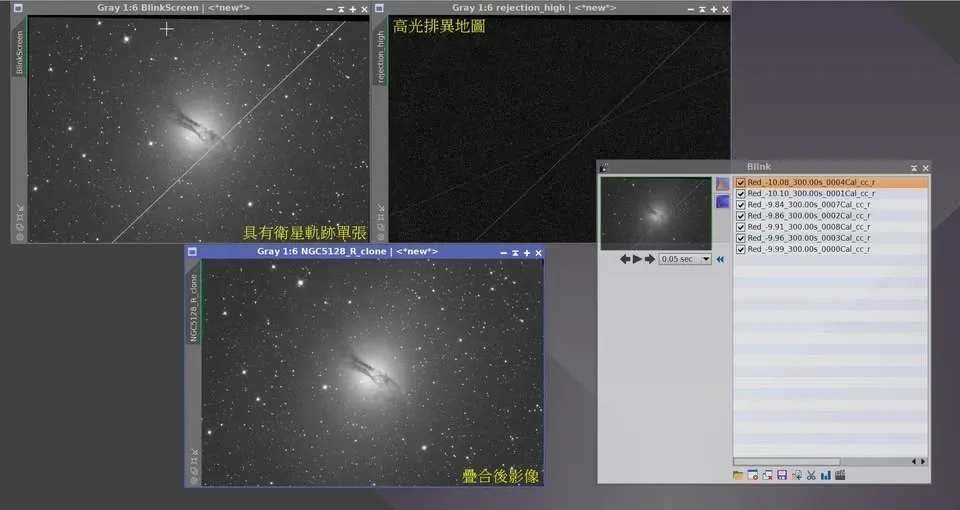
One of 7 frames has a satellite trail cutting across the target, automatically rejected via strict Sigma High parameters

Here’s how: if you have few frames, use an algorithm with stronger rejection power (for example the Sigma Clipping family) and set the Sigma High parameter a bit stricter (say, below 2.5). In one example I had only 7 frames, one of which had a satellite trail cutting across the target; every frame mattered for the signal-to-noise ratio, so with the right parameters (not the software defaults) I let the integration process do the rejection automatically, and the successfully rejected trail shows up in rejection high. Don’t waste a single hard-won pixel.

The Defect-Column Exception: Rejection Can’t Save It

Finally, one exception that rejection can’t save — a CCD’s defect column.

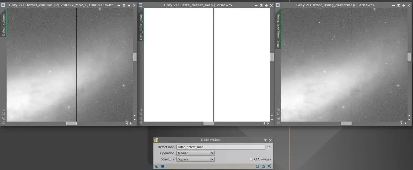
Using a Defect Map to eliminate the CCD defect column, leaving the remainder to rejection

The defect column is too dark and runs the full length; forcing rejection to remove it costs too many good pixels and still works poorly. The right approach is to first build a Defect Map for the camera (take my “Latte” 16803 CCD as an example, with one obvious defect column in the middle of the frame plus three fainter ones), load and apply it to the light frames with the DefectMap process to greatly reduce the defect column’s impact, then let integration rejection easily clean up what’s left. In other words, rejection is the cleanup crew at the end, not an all-powerful first line of defense — defects that call for a dedicated tool still need the right tool first.