Field-Center Offset and Integration Seams

When you accumulate data over multiple nights, or combine data shot with several sets of equipment, the field centers of each set often don’t line up — sometimes because of a difference in the field rotation angle of the gear, sometimes because of a pointing offset for some reason. This leaves obvious seams after integration. The good news: most of the time this situation doesn’t require reshooting — as long as you use the right parameters for registration and integration, the seam can be almost completely eliminated. Don’t waste a single hard-won pixel.

Even a 45-Degree Field Rotation Can Be Seamless

I ran into this problem the very first time I tried combining photos shot with two different sets of equipment: even though it was the same target and the telescope focal lengths were similar, the two cameras’ fields happened to differ by exactly 45 degrees, so the four corners couldn’t overlap, and stacking them directly produced an obvious blending boundary.

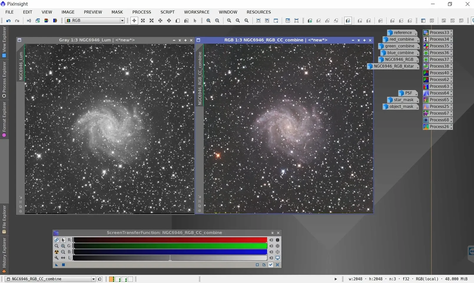
After proper registration and integration, you can’t see any boundary trace at all. One thing to note: all of this holds on one precondition — flat calibration must succeed. The field offset itself has little impact; unless you zoom in a great deal you basically can’t see it, especially with a monochrome camera. For two datasets like this with a 45-degree field rotation difference, you have to zoom carefully to 300% to see any difference in the signal-to-noise ratio at the four corners after integration.

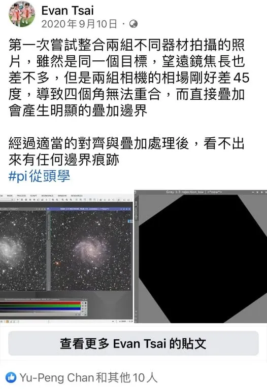
Using Rejection to Eat Up the Non-Overlapping Black Regions

Now for another example of a center offset. While processing M51 I had two sets of images, A and B; in set B the image center didn’t fall on M51 itself, because the OAG was targeting a bright star. After registering set B to set A (which is centered on M51), the areas of set A’s footprint that set B doesn’t cover come out completely black in set B’s registered frames.

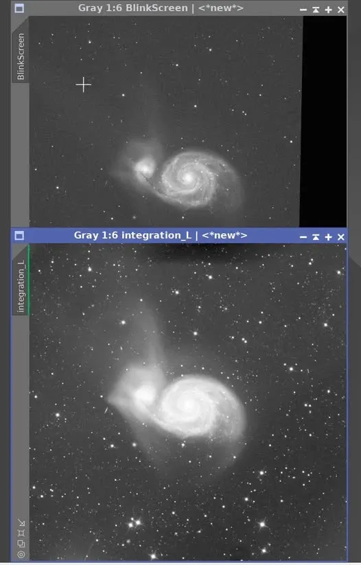
The key is that in the final A/B integration, you choose an appropriate rejection algorithm to reject all those black parts, and the seam becomes completely invisible — even at 400–500% zoom. Plenty of people would think “just reshoot,” but that actually wastes data: set B has 15 frames in the L channel alone, 20 minutes each, and to reshoot to the same position as set A would mean spending at least another 5-plus hours on the L channel. As long as M51 is still within the image range, careful use of preprocessing solves it — why start over?

Don’t Overlook Seams in the Color Channels

When dealing with field offset, there’s another trap that’s easy to overlook: the seam behaves differently in different channels.

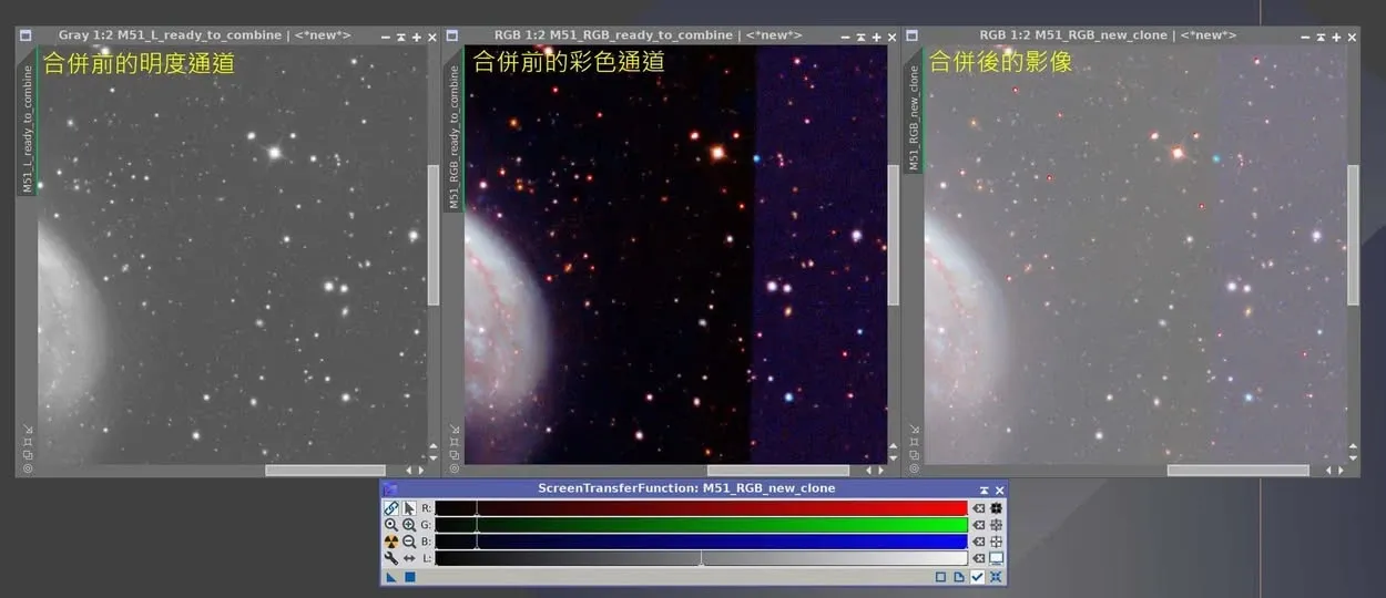
Again, two image sets whose fields don’t overlap: the luminance (L) channel, because the frame count on either side of the boundary is about the same, shows no difference after integration (left image); but in the color channels, the blue channel, because the frame counts on either side of the boundary differ greatly, has a clearly different signal-to-noise ratio, so a boundary appears (middle image). As a result, after the LRGB combine, the poorer signal-to-noise ratio of the blue channel means the final image still shows the boundary (right image).

So the conclusion is clear: the color channels are just as important as the luminance channel, and both affect the final image quality. If either side isn’t handled well, it basically drags down the finished product. Rather than clinging to claims like “a 5-minute L rescued 4 hours of RGB,” honestly handle each channel’s own problems properly — and all of this can actually be verified through software experiments, rather than relying on plausible-sounding anecdotes.